1. Introduction

High-temperature industrial processes, such as metal 3D-printing, laser welding and heat treatment, require continuous real-time monitoring of temperature distribution [1]. During the additive manufacturing process, cyclic heating of the material leads to repeated melting and subsequent solidification, which can cause anisotropic shrinkage of the part layers [2–4]. Thermal deformations resulting from heat transfer between part layers, as well as between the initial layer and the substrate, create a gradient of mechanical stresses. This gradient can lead to deformation of the final product [3–7]. Non-uniform heating and cooling rates contribute to the formation of local defects and disruption of the sample’s microstructure [8–10].

Among the most used materials in metal additive manufacturing (AM) are alloys of the following types: SS316, Ti-6Al-4V, and IN 718. The temperature difference between the liquidus and solidus for these alloys is 40°C, 50°C, and 76°C, respectively [3, 4]. A local decrease in the melt pool temperature comparable to these temperature differences can lead to the formation of various types of defects within the part volume. Therefore, development of tools for monitoring temperature distribution in the working zone is a critical task for improving the quality of AM and other high-temperature industrial processes.

Point-measurement infrared (IR) pyrometry, which averages temperature values over a finite spatial area [11, 12], is the fastest method for temperature monitoring during AM. However, this method cannot be applied for assessment of the nature of spatial temperature distribution without additional spatial scanning. Existing solutions based on imaging radiometric IR pyrometers enable the acquisition of two-dimensional spatial temperature distributions during AM process monitoring [13, 14]. However, the inability to account for spatial and spectral emissivity non-uniformity increases measurement error [15]. Additionally, imaging in the long-wave IR range leads to a significant decrease in spatial resolution [16]. Spectral thermal mapping methods implemented using spectral imaging systems operating in the visible and near-IR ranges are free from these limitations. These methods include two-wavelength imaging pyrometry [17] as well as multispectral [18] and hyperspectral imaging [19]. Two-wavelength visible and near-IR pyrometers are relatively simple and affordable technical solutions. However, the measurement error inherent for this type of devices significantly increases when the object temperature is below 2000 °C. Hyperspectral (HS) systems provide the lowest thermal mapping error across a wide range of object temperatures. However, regardless of their operating principle, these systems acquire a complete data array through spatial or spectral scanning. This feature reduces their temporal resolution and complicates their application for thermography of non-stationary objects and processes. Multispectral (MS) imaging-based methods provide a compromise solution capable of ensuring high temporal resolution due to the absence of spatial or spectral scanning. They also offer acceptable spatial resolution, which decreases proportionally to the increase in the number of spectral channels [20]. However, temperature measurement error under conditions of limited spectral channel numbers is significantly influenced by their characteristics, including the position, width and shape of the transmission function.

The previously proposed approach based on a four-wavelength multispectral camera [21] for monitoring temperature distribution, which accounts for spatial and spectral emissivity inhomogeneities, demonstrates measurement error comparable to other existing spectral methods. This study focuses on selecting optimal characteristics of spectral filters used in each camera channel. These characteristics are designed to reduce temperature measurement error.

2. Materials and methods

All heated bodies serve as sources of thermal radiation, whose spectral and energetic characteristics depend on the temperature T and emissivity ε of the body [22]. When radiation is in thermodynamic equilibrium with the matter, its spectral radiance can be described by Planck’s formula:

where h = 6,63×10^-34kg·m²·s⁻¹ – Planck constant, k = 1,38×10²³J·K – Boltzmann constant, ñ = 3×10⁸ m/s – speed of light in vacuum.

In most cases, remote temperature monitoring methods are based on approximating the acquired values to the nearest curve (1) by selecting optimal values of T and ε. When the object temperature exceeds 3000 °C and the maximum spectral density falls within the visible wavelength range, the Wien approximation is often used to simplify calculations [16]. However, at lower temperatures, the mentioned approach should only be employed for approximate initial estimation.

The thermal radiation spectrum of a monitored object depends on both T and ε, where characterizes the deviation of the object’s spectrum from that of a black body (BB) and is determined by the physical properties of the object’s surface. Reference values of emissivity ε are known for certain materials across broad temperature and spectral ranges. However, a universal computational model describing the ε(λ,T) dependence currently does not exist, and complex multicomponent material configurations remain undocumented. This lack of comprehensive data leads to increased temperature measurement errors. Imaging radiometric IR pyrometry assumes spatial homogeneity of ε across the entire field of view. This assumption introduces significant measurement errors due to the inability to account for ε variations in each pixel of the recorded image [16]. During spectral thermal mapping, an array of images I(x,y,λ) is recorded at different wavelengths, followed by temperature T(x,y) fitting for each pixel. Approximation is typically performed using various numerical optimization methods, including least squares method [23] and Nelder-Mead method [24]. Simultaneous optimization of T and ε allows the individual choice of ε(x,y,λ) values for each pixel to reduce temperature measurement error. However, the significant reduction in spectral data during MS imaging compared to HS imaging affects approximation accuracy. Therefore, it is essential to consider in more detail the criteria for optimal selection of MS imaging spectral channel characteristics.

2.1 Experimental setup

 

Fig. 1. Experimental setup layout. AS – aperture stop, BB – black body source, HS – hyperspectral camera.

 

The initial data for determining optimal spectral filter characteristics were obtained from sets of spectral images of the BB source output aperture, acquired using an experimental setup (see Figure 1). During stepwise heating of the BB source (Metropir Gelios) within the temperature range of ∆ T = 900–1500 °C with 100 °C increments. After stabilizing each intermediate temperature value, HS camera (Specim IQ) positioned coaxially with the BB output window at 150 mm acquired an array of spectral intensity values I(x,y,λ) at the specified temperature. To optimize the use of the HS camera detector dynamic range, a circular aperture with 2 mm diameter was installed in front of the first lens surface. The experimental setup described enabled the creation of a dataset containing black body (BB) radiation intensity values across 204 spectral channels. These channels were identical in terms of optical configuration and detector parameters, ensuring their accurate comparison.

The previously developed four-wavelength MS camera [21] utilized spectral filters with central wavelengths of 620 nm, 660 nm, 780 nm, and 840 nm, and corresponding bandwidths (full width on half maximum – FWHM) of 21 nm, 39 nm, 37 nm, and 30 nm, respectively. During subsequent numerical simulations, combinations of hyperspectral (HS) camera spectral channels were used to simulate the sets of spectral images obtained by the four-wavelength MS camera.

2.2 Preliminary data processing

The preliminary data processing included correction of spatial and spectral inhomogeneities caused by characteristics of the optical system and detector sensitivity of the HS camera. Additional processing steps involved intensity correction based on exposure time and background filtering. To determine spatial brightness inhomogeneity within the field of view of HS camera, imaging of the integrating sphere output window (Spectra-FT-2300-W, Labsphere) was performed. This device provided uniform luminance across the field of view within the operational spectral range. Spectral sensitivity of the HS camera was determined through image acquisition simulating narrowband radiation sources with known intensity with a monochromator (M266i–IV, Solar Laser Systems) and a plasma broadband radiation source (XWS-65, ISTEQ). Additionally, the array of BB spectral intensity values obtained at T = 900°C was used to calculate correction factors and account for residual spectral sensitivity inhomogeneity of the HS camera. An optimal exposure time was selected to maintain acquired signal values within the linear response range of the HS camera detector for each temperature change of the BB. The intensity normalization was performed to ensure correct correlation between spectral data arrays. Background filtering using threshold binarization was conducted considering the image at wavelength λ = 900 nm as the baseline.

To estimate temperature, spectral characteristics were averaged over pixels corresponding to the BB output aperture. Subsequently, an approximation method using the Planck function (1), detailed in [21], was applied. An iterative search was implemented for all possible unique four-element wavelength combinations under the condition λ₁ < λ₂ < λ₃ < λ₄, where λᵢ represents the maximum position of the i-th spectral channel transmission function. Spectral intensity values from the same image regions were selected based on these combinations, followed by similar temperature estimation procedures. During channel width modelling the spectral data was approximated using a Gaussian function within the specified range, the area under the approximation curve was calculated. The width variations were accounted for by normalization on the area under the transmission function curve of the corresponding channel. To obtain a quantitative estimate of the accuracy of temperature predictions, a set of metrics [25] was employed: MAE (Mean Absolute Error, °C); MAPE (Mean Absolute Percentage Error, %); RMSE (Root Mean Square Error, °C); Bias (Mean bias, °C) and R² (Coefficient of determination).

2.3 Optical system radiometric calculation

The transmission function maxima positions and bandwidths of spectral filters also should be accounted for during the selection of the image sensor (IS) and lenses, as they are directly related to the energy capacity of the optoelectronic system and require a specific level of IS sensitivity within the specified wavelength range. An additional condition for the optimal filter bandwidth selection is the exposure time required to achieve the necessary signal-to-noise ratio. The solution to this problem is based on the optical system radiometric calculation, which determines the relationship between the filter bandwidth and the minimum possible IS exposure time. The minimal exposure time is directly related to the frame acquisition rate. A general pipeline for the radiometric calculation of an individual MS camera channel is presented.

A melt pool with dimensions X × Y = 10 × 10 mm was selected as the object observed by the MS camera. The melt may be heated to three temperatures T equal to 900 °C, 1400 °C, and 1900 °C.

The following assumptions are proposed. The object emits as BB and a Lambertian radiation source. The object is located at a distance a = 400 mm from the MS camera lenses. The considered MS camera configuration includes identical lenses with focal length f′ = 35 mm and relative aperture D/f′ = 1:3 (entrance pupil diameter D ≈ 11.67 mm) and a silicon-based IS (The Imaging Source DMK 33GX264) with pixel size A_x × A_y = 3.45 × 3.45 μm and total pixel count 2048 × 2448. As the MS camera has 4 separate channels, pixel count per channel is approximately 900 × 1100 and an individual channel image size is 3.105 × 3.795 mm. The lens transmittance τ_lens(λ) = 0,6 remains constant in the spectral filter transmission function τ_filter(λ) which is approximated by the gaussian curve with a peak value of 0,9.

First, the paraxial geometric parameters of the system under consideration are determined. In accordance with a the thin lens formula [26], the distance from the lens to the image a’ is:

The linear magnification β of an individual channel:

The area A_pixel of the pixel projection in the object space:

Radiant flux Ô_pixel acquired by a single pixel:

where L_e(λ,T) is an object spectral radiance (1).

Considering radiant flux acquired by a single pixel the minimal exposure time t_min may be estimated. Detection of a signal by the IS pixel requires the number of photoelectrons to exceed the IS noise level accounting the IS quantum efficiency QE(λ). The number of photoelectrons may be expressed using the accumulated photon energy E_photon(λ). The photon energy at individual wavelengths λ is calculated using the following formula:

Total number of photoelectrons for a single pixel irradiated in a spectral range Δλ:

The minimal exposure time may be assessed as follows:

where N_min is the minimal number of photoelectrons required for signal-to-noise ratio 1; SNR is the desired signal-to-noise ratio. For a chosen IS model the intrinsic noise does not exceed 3 photoelectrons, and the pixel capacity is approximately 10000 photoelectrons. Thus, signal-to-noise ratio may be assigned as SNR = 1000.

Substituting (5) and (6) into (7), and then (7) into (8), one can obtain the equation that associates the minimum exposure time with the filter bandwidth:

3. Results

Since the black body (BB) model temperature is set in degrees Celsius, temperature values and their errors are also presented in degrees Celsius in this section. For numerical analysis, the obtained values were converted to absolute temperature. Subsequently, an inverse conversion was performed for graphical representation.

3.1 Numerical analysis of HS and MS configurations

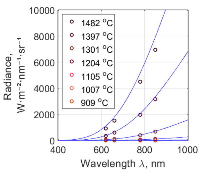
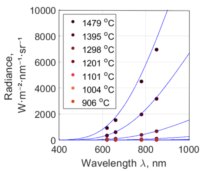
Figure 2 demonstrates the results of temperature estimation based on averaged BB spectra within the considered range, using data from the HS camera and the previously proposed MS camera with channel central wavelengths of 620 nm, 660 nm, 780 nm, and 840 nm. We presented three bandwidth models: negligible bandwidth, equal bandwidth of 30 nm for each channel and using actual bandwidths of 21 nm, 39 nm, 37 nm, and 30 nm for respective channels.

 

Fig. 2. Comparison of temperature estimates for HS (a) and MS configurations with negligible bandwidth (b), fixed equal bandwidth (c) and actual bandwidth (d)

 

Obtained temperature accuracy metrics for HS and MS camera configurations are shown in Table 1.

Table 1 – Temperature accuracy metrics for HS and MS configurations

Camera configuration	MAE, °C	MAPE, %	RMSE, °C	Bias, °C	R2
HS camera	4,9	0,4	6,8	-2,5	0,9988
MS camera ( negligible bandwidth)	6,8	0,5	10,5	-6,3	0,9973
MS camera ( equal bandwidth)	6,3	0,5	9,0	-2,3	0,9980
MS camera (actual bandwidth)	7,9	0,7	10,0	0,7	0,9975

3.2 Spectral channel positions optimization

As a result of iterative search through unique combinations of 4 spectral channels with central wavelength positions ranging from 400 to 1000 nm in 10 nm steps, histograms (Fig. 3) were obtained. These histograms demonstrate the frequency of occurrence of particular channels in combinations that provide relative temperature estimation errors of less than 0.5%, 1%, and 5%.

 

a)
b)
c)

Fig. 3. The occurrence of spectral channel positions in combinations providing MAPE lower than 0,5% (a), 1% (b) and 5% (c).

 

The analysis of the obtained distributions shows that as the error threshold decreases, the prominence of spectral regions most critical for estimation accuracy increases. When reducing the permissible error to 0.5% (Fig. 3a), channels with wavelengths between 680 nm and 720 nm appear particularly frequently in optimal combinations. Certain near-infrared (NIR) channels, specifically 760 nm, 840 nm, and 950 nm, are also commonly included in optimal combinations. This indicates that the mentioned central wavelengths provide high information content for temperature estimation. The short-wavelength part of the spectrum (λ ≤ 600 nm) does not participate in combinations providing low relative error, confirming its limited contribution to the task at hand. Specific channel combinations that provide minimal relative error values are presented in Table 2.

Table 2 – Channel central wavelength combinations providing the lowest temperature relative error values.

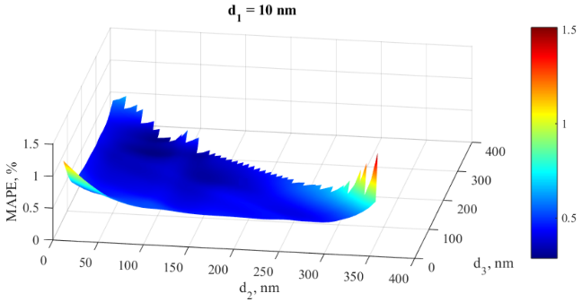
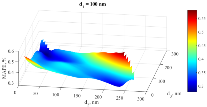
To visualize the distribution of relative temperature estimation error in the four-dimensional space of channels with wavelengths λ_₁, λ_₂, λ_₃, and λ_₄, several methodological steps were implemented. First, the spectral range from 400 to 600 nm was excluded from consideration, as analysis of the histograms demonstrated that this range did not contribute to improving temperature estimation accuracy. Next, dimensionality reduction was achieved by calculation of distances between channel positions. One of the distances was fixed to further simplify the representation. 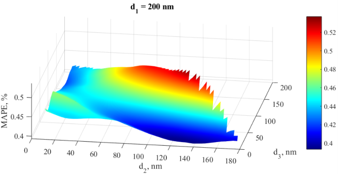This approach enabled the error to be represented in three-dimensional space (Figure 4), where its variation is shown as a color map. In this representation, d_₁ corresponds to the distance between the first and second channels, d_₂ represents the distance between the second and third channels, and d_₃ indicates the distance between the third and fourth spectral channels. To further reduce data dimensionality and simplify the visualization, λ_₁ was fixed at 600 nm.

 

Fig. 4. Dependencies of the temperature relative error on the distance between channel central wavelengths obtained with fixed d₁; 10 nm (a), 50 nm (b), 100 nm (c) and 200 nm (d).

 

Since the error variations are significant through d_₁ distances, their value range is not provided to enhance the contrast of the distribution. The analysis of the obtained distributions demonstrates that at small d_₁ values, considerable errors exceeding 1.5% are observed at extreme values of d_₂ and d_₃. As d_₁ increases, the error significantly decreases, reaching a minimum at d_₁ = 200 nm, and becomes less sensitive to changes in the remaining distances. All diagrams demonstrate presence of feature regions of optimal d_₂ and d_₃ combinations corresponding to minimal relative error, which can be utilized for selecting the configuration of spectral channels.

3.3 Spectral channel bandwidth optimization

To investigate the influence of spectral channel bandwidth Δλ on temperature estimation, their central positions were fixed according to the optimal combination in terms of minimizing relative error — 690 nm, 700 nm, 720 nm, and 910 nm (Table 2). The values of the selected metrics have been compiled in Table 3.

Table 3 – Metric values for comparing spectral channels with fixed position and bandwidth variation.

Table 3 demonstrates the significant decrease of temperature estimation accuracy with increasing spectral channel bandwidth (Δλ). At small Δλ values (5–10 nm), metrics such as Mean Absolute Error (MAE) and Root Mean Square Error (RMSE) exhibit the lowest values.

At these narrow bandwidths, the coefficient of determination (R²) approaches 1, indicating high-quality model performance. However, as the bandwidth increases to 100 nm, errors grow substantially: MAE reaches 33.5 °C, RMSE reaches 35.1 °C, and R² decreases to 0.9691, signaling a deterioration in model-data agreement. The error bias (Bias) transitions from negative values at narrow channels — indicating underestimation of temperature — to significant positive values at wide channels, suggesting systematic overestimation of results. These findings indicate that the use of narrowband spectral channels with bandwidths up to 20–30 nm is preferable for accurate temperature estimation. Conversely, expanding the bandwidth beyond 50 nm introduces considerable errors and limits the practical applicability of the method.

However, it is not feasible to reduce the bandwidth to an infinitesimally small size. According to the described radiometric calculation methodology, two sets of spectral filters installed in front of the lenses are considered for analysis. The first set comprises filters with central wavelengths λ_c of 690 nm, 700 nm, 720 nm, and 910 nm, while the second set includes filters with central wavelengths of 620 nm, 660 nm, 780 nm, and 840 nm. The primary objective of the calculation is to determine the optimal bandwidth (FWHM) for each filter within both sets. 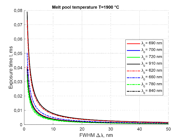By substituting initial values into equation (9) for the given example, the minimal exposure time t_min is calculated for bandwidth values Δλ up to 50 nm. As a result, the diagrams illustrating the dependence of t_min on Δλ for selected object temperatures are obtained. These diagrams represent two distinct configurations: the channel combination utilized in the MS camera prototype and the optimal channel combination derived from numerical calculation. The corresponding dependencies are represented in Figure 5.

The radiometric calculation data for the MS camera demonstrate that the exposure time is inversely proportional to the bandwidth, following the relationship Δλ~1/t_min. As shown in Figure 5, when the filter bandwidth ranges from 5 to 20 nm, the values of minimal exposure time for the IS with different filters exhibit a sharply nonlinear decrease as the filter bandwidth increases. Additionally, it is important to note that filter bandwidths less than 10 nm are unacceptable when operating near the boundaries of the IS sensitivity range, leading the exposure time to exceed 50 ms and making real-time temperature distribution monitoring impossible. Thus, it is recommended to use filters with bandwidths exceeding 20 nm, where the relationship between exposure time and filter bandwidth becomes approximately linear. This ensures both practical feasibility and effective real-time temperature monitoring capabilities.

 

a)	b)
c)

Fig. 5. Dependencies of minimal exposure time on spectral filter bandwidth for melt pool temperature 900 (a), 1400 (b) and 1900 (c) ℃

4. Discussion

The conducted analysis demonstrated that HS imaging enables highly accurate temperature estimation based on absolute evaluation metrics. Specifically, the minimum observed values of MAE (4,9°C), MAPE (0,4%), and RMSE (6,8°C), along with a coefficient of determination R² of 0,9988, indicate a strong concordance between the experimental data and the Planck model, provided that high spectral resolution data are available. However, the high cost, the need for spectral or spatial scanning, and the large volume of data processing make HS cameras impractical for real-time monitoring of non-stationary objects and processes [28]. Moreover, the relative error in temperature estimation derived from simulated MS data using optimally positioned spectral channels was found to be even lower (MAPE = 0,2%). This improvement may be attributed to the inclusion of spectral bands exhibiting the highest sensitivity to variations in spectral radiance at typical object temperatures (Fig. 3). In contrast, the estimation derived from HS data may have been adversely affected by spectral edge regions, where the signal-to-noise ratio is reduced due to diminished detector sensitivity [29]. These findings suggest that the strategic selection of optimal central wavelengths for a limited number of spectral channels can yield a more stable and accurate temperature estimation. Furthermore, reformulating the optimization task in a parameter space defined by inter-channel distances (d₁, d₂, d₃) facilitated dimensionality reduction. It enabled the visualization of regions corresponding to optimal channel configurations (Fig. 4). These results underscore the significance of spectral separation as a crucial factor in determining the accuracy of MS-based temperature estimation.

The MS camera under consideration comprises four independent spectral channels, each forming an image on a separate sector of the IS. Variations in the incident radiative flux across spectral channels may lead to dynamic range limitations of the IS, thereby compromising the contrast of spectral images. To mitigate this issue, it is necessary to adjust the camera’s operational mode. The system uses two primary acquisition strategies:

1. Uniform Integration Mode: The spectral filter characteristics are selected so that the minimum integration time required to achieve the desired signal-to-noise ratio is approximately equal across all channels. This approach aligns the channels within a standard dynamic range, allowing simultaneous acquisition of images across all spectral bands. While this mode provides enhanced temporal resolution, it may introduce greater temperature estimation error due to broader filter bandwidths.

2. Sequential Exposure Mode: A sequence of frames (typically 2 to 4) is acquired, each with different integration times. Integration time for each frame is optimized to achieve the target signal-to-noise ratio for the corresponding spectral channel. During subsequent processing, the system selectively extracts the relevant channel data from each frame. Although this method reduces temporal resolution, it yields improved accuracy in temperature measurement.

In the presented study, considering the application of the first operational mode and accounting for the influence of filter bandwidth on both temperature measurement accuracy and IS integration time, the optimal filter bandwidth is recommended to be in the range of 20 to 30 nm.

5. Conclusion

The results of this study confirm the high efficacy of temperature estimation, a characteristic of AM processes, based on spectral radiance measured by an MS imaging system. The analysis identified optimal spectral channels for minimizing estimation errors within the 680–720 nm range, as well as specific bands in the near-infrared region, particularly at 760, 840, and 950 nm. With selected wavelengths at 690, 700, 720, and 910 nm and spectral bandwidths in the range of 20–30 nm, the MS camera achieved temperature estimation accuracy comparable to that of a HS system (MAE ≈ 4 °C, MAPE ≈ 0,3%), while significantly outperforming it in terms of computational efficiency, acquisition speed, and implementation simplicity.

The study provides guidelines for selecting spectral bandwidths. We demonstrated that increasing the bandwidth beyond 50 nm substantially increases the estimation error, while excessively narrowing it causes prohibitively long integration times, especially under conditions of reduced detector sensitivity. As such, the selection of bandwidth must reflect a trade-off between spectral selectivity and acceptable integration time.

These findings support the development of compact, high-performance temperature monitoring systems based on a limited number of narrowband spectral channels. Such systems can achieve accuracy on par with HS-based approaches while offering greater adaptability to the practical requirements of modern manufacturing environments. These systems allow real-time monitoring of thermal variations during processes such as metal additive manufacturing, laser welding, and thermal treatment.

Acknowledgments

The study was supported by a grant from the Russian Science Foundation No. 24-79-10239 (https://rscf.ru/en/project/24-79-10239/).

References

1. Patterson T., Hochanadel J., Sutton S., Panton B., Lippold J. A review of high energy density beam processes for welding and additive manufacturing applications / Welding in the World, 2021, Vol. 65, No. 7, pp. 1235-1306.

2. Paul R., Anand S., Gerner F. Effect of Thermal Deformation on Part Errors in Metal Powder Based Additive Manufacturing Processes / Journal of Manufacturing Science and Engineering, 2014, Vol. 136, No. 3, P. 031009.

3. Mukherjee T., Manvatkar V., De A., DebRoy T. Mitigation of thermal distortion during additive manufacturing / Scripta Materialia, 2017, Vol. 127, pp. 79–83.

4. Heigel J.C., Michaleris P., Palmer T.A. In situ monitoring and characterization of distortion during laser cladding of Inconel® 625 / Journal of Materials Processing Technology, 2015, Vol. 220, pp. 135–145.

5. Bian P., Shao X., Du J. Finite Element Analysis of Thermal Stress and Thermal Deformation in Typical Part during SLM / Applied Sciences, 2019, Vol. 9, No. 11, P. 2231.

6. Fyrillas M.M., Papadakis L. Transient Powder Melting in SLM Using an Analytical Model with Phase Change and Spherical Symmetry in a Semi-Infinite Medium / Journal of Manufacturing and Materials Processing, 2019, Vol. 3, No. 2, P. 50.

7. Dunbar A.J., Denlinger E.R., Heigel J., Michaleris P., Guerrier P., Martukanitz R., Simpson T.W. Development of experimental method for in situ distortion and temperature measurements during the laser powder bed fusion additive manufacturing process / Additive Manufacturing, 2016, Vol. 12, pp. 25–30.

8. Vafadar A., Guzzomi F., Rassau A., Hayward K. Advances in Metal Additive Manufacturing: A Review of Common Processes, Industrial Applications, and Current Challenges / Applied Sciences, 2021, Vol. 11, ¹ 3, P. 1213.

9. DebRoy T., Wei H.L., Zuback J.S., Mukherjee T., Elmer J.W., Milewski J.O., Beese A.M., Wilson-Heid A., De A., Zhang W. Additive manufacturing of metallic components – Process, structure and properties / Progress in Materials Science, 2018, Vol. 92, pp. 112–224.

10. Kok Y., Tan X.P., Wang P., Nai M.L.S., Loh N.H., Liu E., Tor S.B. Anisotropy and heterogeneity of microstructure and mechanical properties in metal additive manufacturing: A critical review / Materials & Design, 2018, Vol. 139, pp. 565–586.

11. Belikov R., Merges D., Varentsov D., Major Z., Neumayer P., Hesselbach P., Schanz M., Winkler B. Fast Multi-Wavelength Pyrometer for Dynamic Temperature Measurements / International Journal of Thermophysics, 2024, Vol. 45, No. 2, P. 29.

12. Mamuschkin V., Haeusler A., Engelmann C., Olowinsky A., Aehling H. Enabling pyrometry in absorber-free laser transmission welding through pulsed irradiation / Journal of Laser Applications, 2017, Vol. 29, No. 2, P. 022409.

13. Vuelban E.M., Girard F., Battuello M., Nemecek P., Maniur M., Pavlasek P., Paans T. Radiometric Techniques for Emissivity and Temperature Measurements for Industrial Applications / International Journal of Thermophysics. 2015. V. 36, No. 7. P. 1545–1568.

14. Everton S.K., Hirsch M., Stravroulakis P., Leach R.K., Clare A.T. Review of in-situ process monitoring and in-situ metrology for metal additive manufacturing / Materials & Design, 2016, Vol. 95, pp. 431–445.

15. Mazzarisi M., Angelastro A., Latte M., Colucci T., Palano F., Campanelli S.L. Thermal monitoring of laser metal deposition strategies using infrared thermography / Journal of Manufacturing Processes, 2023, Vol. 85, pp. 594–611.

16. Grujic K.A. Review of Thermal Spectral Imaging Methods for Monitoring High-Temperature Molten Material Streams / Sensors, 2023, Vol. 23, No. 3. P. 1130.

17. Myers A.J., Quirarte G., Ogoke F., Lane B.M., Uddin S.Z., Farimani A.B., Beuth J.L., Malen J.A. High-resolution melt pool thermal imaging for metals additive manufacturing using the two-color method with a color camera / Additive Manufacturing, 2023, V. 73. P. 103663.

18. Poissenot-Arrigoni C., Marcon B., Rossi F., Fromentin G. In-Situ Pixel-wise Emissivity Measurement Using a Multispectral Infrared Camera / Journal of Imaging, 2023, Vol. 9, No. 10, P. 198.

19. Staudt T., Eschner E., Schmidt M. Temperature determination in laser welding based upon a hyperspectral imaging technique / CIRP Annals, 2019, Vol. 68, No. 1. pp. 225–228.

20. Shogenji R., Kitamura Y., Yamada K., Miyatake S., Tanida J. Multispectral imaging using compact compound optics / Optics Express, 2004, Vol. 12, No. 8, P. 1643.

21. Bykov A., Zolotukhina A., Poliakov M., Belykh A., Asyutin R., Korneeva A., Batshev V., Khokhlov D. Four-Wavelength Thermal Imaging for High-Energy-Density Industrial Processes / Journal of Imaging, 2025, Vol. 11, No. 6, P. 176.

22. Handbook of thermophysical properties of solid materials. / Goldswith A., Waterman T. E., Hirschhorn H. J. New York: Macmillan, 1961. 4300 p.

23. Andreic Z. Distribution temperature calculations by fitting the Planck radiation curve to a measured spectrum / Applied Optics, 1992, Vol. 31, No. 1, pp. 126–130.

24. Lagarias J.C., Reeds J.A., Wright M.H., Wright P.E. Convergence Properties of the Nelder-Mead Simplex Method in Low Dimensions / SIAM Journal on Optimization, 1998, Vol. 9, No 1, pp. 112–147.

25. Chicco D., Warrens M. J., Jurman G. The coefficient of determination R-squared is more informative than SMAPE, MAE, MAPE, MSE and RMSE in regression analysis evaluation / PeerJ Computer Science, 2021, Vol. 7, P. e623.

26. Theory of optical systems: a textbook for students of instrument-making specialties at universities. / Zakaznov N. P., Kiryushin S. I., Kuzichev V. I. Moscow: Mashinostroenie, 1992. 448 p. [in Russian]

27. The Imaging Source – DMK33GX264 Datasheet. 2025. URL: https://s1-dl.theimagingsource.com/api/2.5/packages/documentation/datasheet/ds_dmk33gx264/4935baf8-e93e-5b98-805d-333bab61e7ad/ds_dmk33gx264.en_US.pdf (access date: 14.07.2025).

28. Cheng M.-F., Mukundan A., Karmakar R., Valappil M. A. E., Jouhar J., Wang H.-C. Modern Trends and Recent Applications of Hyperspectral Imaging: A Review / Technologies, 2025, Vol. 13, No. 5, P. 170.

29. Rasti B., Scheunders P., Ghamisi P., Licciardi G., Chanussot J. Noise Reduction in Hyperspectral Imagery: Overview and Application / Remote Sensing, 2018, Vol. 10, No. 3, P. 482.