1. Introduction

The objective of the study is to propose a technique for visualizing the results of short text clustering using the GSDMM algorithm to facilitate the analysis of the results and the selection of hyperparameters of this algorithm and dictionary.

Why GSDMM? It is the most popular short text clustering algorithm on GITHUB. Additionally, a query on ScienceDirect for “Title, Abstract, Keywords: ‘short text’ clustering algorithm” returns 27 results across all years. In the exported RIS file of these 27 records, GSDMM appears 12 times in 6 papers, LDA appears 17 times in 6 papers, “suffix tree” appears 4 times in one paper. But GSDMM is close to LDA, but for short texts — one topic per text.

BERTopic [1] is also widely used for studying text topics, but it is not an algorithm, but a whole sequence of procedures. According to the developer of the program “By default, the main steps for topic modeling with BERTopic are sentence-transformers, UMAP, HDBSCAN, and c-TF-IDF run in sequence.” Even more, UMAP [2] — procedure using its own parameters [3], and “sentence-transformers” is also dependent on the training sample. BERT is suitable for vectorizing short texts on Twitter, but other models may be more appropriate for different text sources. [4]. Even if BERTopic gives good results, the analysis of the influence of the parameters of the procedures at each step on the final results seems questionable, so this program was excluded as an alternative to GSDMM.

Choosing a GSDMM implementation. According to the query “https://github.com/search?q=short%20text%20clustering&type=repositories”, the algorithm GSDMM: Short Text Clustering implemented by Ryan Walker has the highest rating and is implemented in both Python and Rust [5]. It should be noted that there are also implementations of this algorithm in Java and GO.

Visualization of clustering results using the GSDMM algorithm. A query on GITHUB “GSDMM” returns 46 outputs, but the visualization of the results of this algorithm is only implemented in two Python projects: “center-for-humanities-computing/tweetopic” [6] and “Illias-b/Natural-Language-Processing” [7]. In both cases, the results are presented in the form of term clouds and bar charts.

Note: The Center for Humanities Computing is notable for publishing the journal Computational Humanities Research, showcasing cutting-edge research at the intersection of computational methods and the humanities.

Note: The authors of the GSDMM algorithm [8] in the introductory part of their paper discuss and justify the need for its creation by the differences between clustering short texts and clustering regular texts. Also, short texts are more often related to a single topic, while long texts can cover several topics.

The advantage of the two visualization approaches described above is that they can be done quickly. A number of parameters can be set, but the implementation procedures remain the same. This advantage is also the main disadvantage — lack of flexibility in the choice of procedures at each step, especially in text preparation, dictionary selection and bar chart construction.

What is good for constant monotonous work is not always suitable for research work, where, in my opinion, it is more appropriate to use the well-known approach: the program does one thing, but does it well. In this case, at each stage it is easier to analyze the result, adjust parameters and choose procedures. The work takes more time, but it allows you to analyze the whole process in more depth. For example, in this study, the bar chart is displayed not by the ratio of the occurrence of a term in one cluster to its total occurrence, but by the difference between the occurrence of a term in one particular cluster and other individual clusters. The flexible text preprocessing and dictionary selection for GSDMM were also used.

The novelty of this study lies in the choice of bar chart for visualizing the results of text clustering using GSDMM and comparing the topics of clusters with the clustering based on the co-occurrence of keywords.

The following sections discuss the detailed implementation of the above.

2. Materials and methods

The source of the short texts was bibliometric records on the “Visualization” topic exported from Scopus, the scientific abstracts and citations database on November 12, 2024.

In order to focus on the issue of visual presentation of clustering results, this paper only uses the Author keywords as short texts. The use of titles and abstracts as short texts requires a more detailed choice of their preprocessing and is not considered in this paper.

Bibliometric data were exported on request: (TITLE-ABS-KEY(“Visual Analytics” OR “Data Visualization” OR “Information Visualization” OR “Visualization Technique” OR “Visual Representations” OR “Visual Languages” OR “Visualization Tools” OR “Visual Exploration” OR “Visualization System” OR “Visual Analysis” OR “Interactive Visualizations” OR “Flow Visualization”) AND (LIMIT-TO (DOCTYPE,”ar”))  AND (LIMIT-TO (LANGUAGE,”English”))  AND (LIMIT-TO (SUBJAREA,”ENGI”) OR LIMIT-TO (SUBJAREA,”COMP”) OR LIMIT-TO (SUBJAREA,”ENER”))  AND (LIMIT-TO (PUBYEAR,2020) OR LIMIT-TO (PUBYEAR,2021) OR LIMIT-TO (PUBYEAR,2022) OR LIMIT-TO (PUBYEAR,2023) OR LIMIT-TO (PUBYEAR,2024))). 16486 records were received.

Gibbs Sampling Dirichlet Multinomial Mixture (GSDMM) implementation in Rust was used [5] with parameters: 𝛼 = 0.002, 𝛽 = 0.5, 𝐼 = 1000, 𝐾 = 30.

The parameters were chosen experimentally in order to obtain no more than 10 clusters without very small ones. The purpose of the paper was to visualize the clusters, not to study their themes in detail. For the latter, it would be useful to focus on more clusters and other algorithm parameters.

Here, 𝛼 and 𝛽 are parameters whose meaning is explained below. 𝐾 — is the maximum allowed number of clusters generated by the algorithm. 𝐼 — is the number of iterations.

The large value of 𝛽 = 0.5 is due to the need to increase the size of clusters (to reduce their number), 𝛼 = 0.002 for the rare appearance of new groups, large 𝐾 = 30 and 𝐼 = 1000 are chosen for a longer observation of the convergence to the number of clusters. With these parameters, 9 clusters are obtained.

Note: in the work of the authors of the algorithm [8], Figure 9 shows a decrease in the number of clusters (up to 50 or 100 depending on the Set) as 𝛽 increases from 0.02 to 0.2. The number of clusters less than 10 (9) acceptable for analysis within the scope of this paper was obtained at 𝛽 = 0.5.

In text and figures, cluster numbering is preserved as given by the GSDMM algorithm.

To visualize the results obtained using the GSDMM algorithm, Scimago Graphica [9] is used, which not only provides the ability to export vector graphics, but also the formation of interactive HTML pages that facilitate the understanding of the visualization results. In addition, Scimago Graphica offers great opportunities for handling the parameters of graph construction.

The GSDMM algorithm compares short texts based on the terms in the dictionary. Therefore, the texts and dictionary terms were lemmatized to normalize them.

The difference between the most frequent keywords in a particular cluster and those in other clusters was obtained using SQL queries.

Note: Since the comparison of texts is based on dictionary terms, the same terms may appear in different clusters. In fact, the histograms of the distribution of terms in the clusters are compared.

Note: The algorithm generates a list of clusters starting from a given value, in this case 30, skipping empty clusters, the order for non-empty clusters is preserved in this work.

3. Results and discussions

The overall picture of the author’s keyword clustering using the GSDMM algorithm is presented in Figure 1 in the form of a term cloud, where the color indicates keywords belonging to a particular cluster.

146 records containing the fields: cluster number, keyword and frequency of occurrence of the keyword were used to construct the plot. The list of records was constructed as follows: keywords with the highest frequency of occurrence were selected from each cluster, the number of terms was taken approximately proportional to the cluster size. The exact boundary was determined by the transition of the term occurrence, e.g. records with a frequency of occurrence of term 20 ended and records with a frequency of occurrence of term 19 began. This choice allows for a more balanced representation of terms from each cluster than if the most frequent terms were drawn from the entire list of terms from all clusters.

 

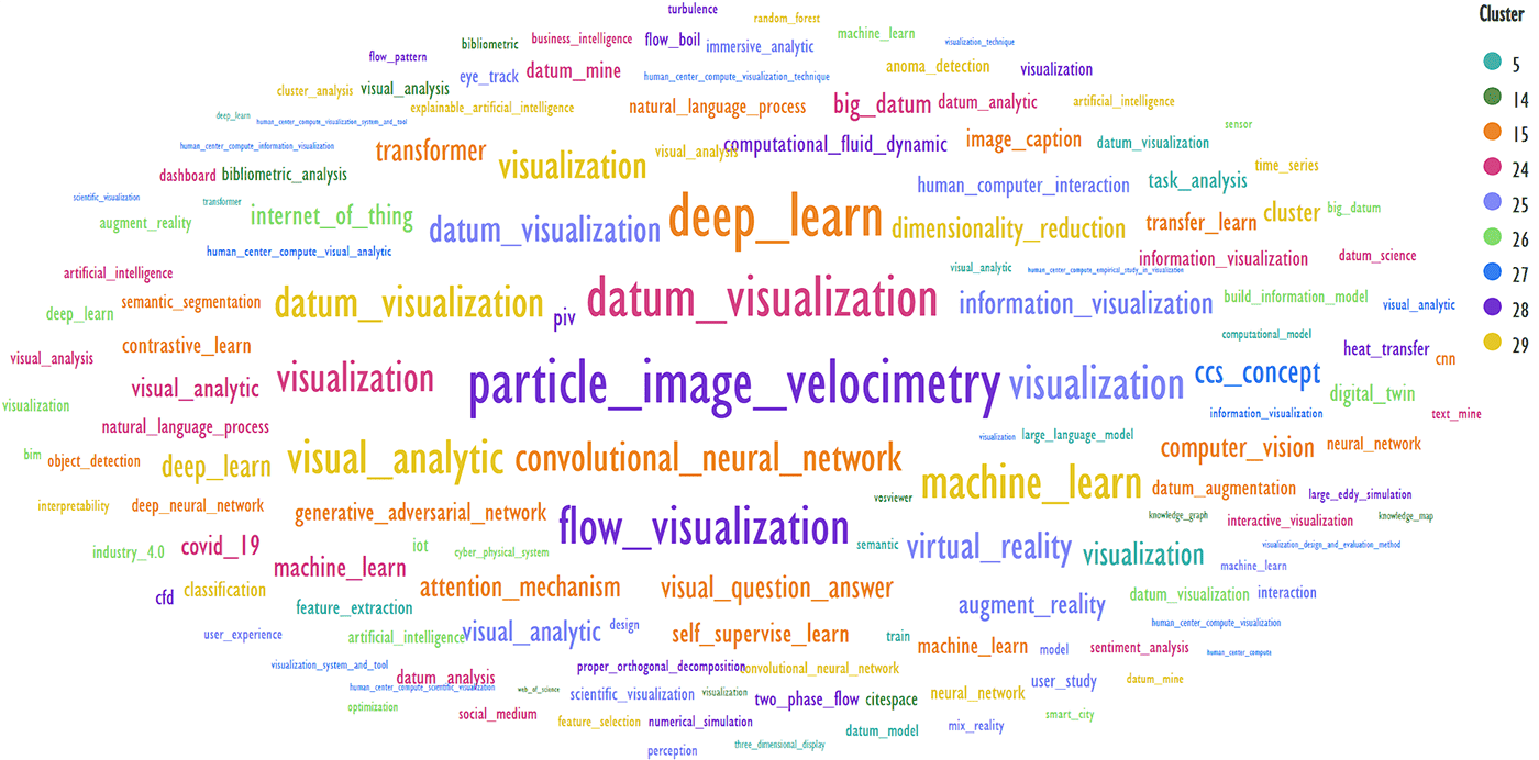
Fig. 1. Author keywords cloud of 146 entries from 9 clusters. Created with Scimago Graphica

 

A more informative representation of the results presented in Figure 1 is given in the form of an interactive Alluvial Diagram available in the archive attached to the article. File — ‘KWsClusterTops4SG-v-2-Alluvial.htm’ (JavaScript is downloaded from Internet)

Terms: ‘particle_image_velocimetry, flow_visualization, computational_fluid_dynamic, two_phase_flow’ occur in only one cluster, so their size in the word cloud is large. The term “visualization” occurs in 8 out of 9 clusters, so the size of this word in the figure is proportional to its occurrence in each cluster. It is typical for document clustering that keywords describing the subject of a cluster can occur in multiple clusters.

These are only the terms included in the 146 records analyzed. A more complete inclusion of keywords is hindered by the readability of the figure in the paper. Choosing the best graphical representation of the term cloud was not the goal of this paper.

3.1 Analyzing the data of each cluster obtained using the GSDMM algorithm

The GSDMM utility generates a file ‘prefix-cluster_descriptions.txt’, which contains for each cluster a list of vocabulary words and their occurrences. The cluster numbers are kept in the original sequence: the first non-empty cluster is labeled as 5, the next cluster as 14, and so on. In addition, the GSDMM utility generates a file indicating the cluster to which each entry/document is assigned and a probability score indicating the degree of correspondence between the entry and the cluster. However, in this particular study, the aim was to select a suitable visual representation of the cluster descriptions based on dictionary words. Therefore, this file was not used in this paper.

To implement visualization, the keywords (words from the dictionary) in a separate cluster, and the other clusters were compared. The data were presented graphically in Figures 2-10.

The archive contains HTML pages with interactive charts that facilitate a fuller understanding of the results.

The occurrence of keywords was compared using the left join operation of this cluster and others. Then the frequency of keywords in this cluster and other clusters was subtracted.

Terms that occurred in the current cluster but did not occur in other clusters were marked as ‘0’ cluster in the graphs to emphasize that they were not clusters other than the current cluster. If there were no such terms, this was labeled as ‘null’ in the graphs. For example, see Figures 2 and 3.

In order to limit the size of the graph, only keywords whose occurrence exceeded a certain threshold, which was different for each cluster, were displayed on the chart. This value was indicated in the caption below the figure.

To emphasize the importance of keywords that occur in the cluster in question but not in other clusters, they can be plotted even if their frequency is lower than the one specified and indicated in the figure caption. For example, Figure 4 shows terms that occur 39 or more times in cluster 15 and also occur in other clusters. However, terms that do not occur in other clusters are shown even if they occur only 10 or more times in cluster 15.

Figure 2 shows the difference between the occurrence of the most frequent keywords in Cluster 5 and the other clusters

 

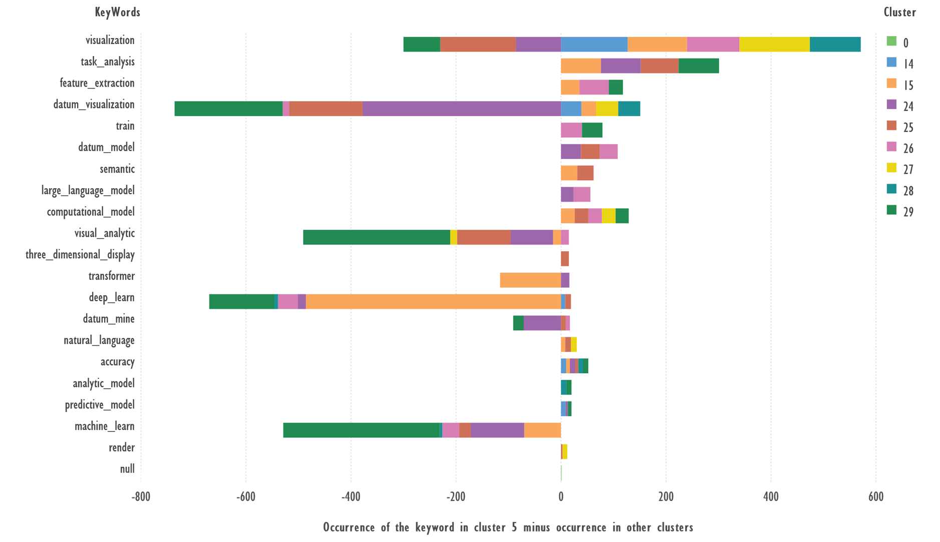
Fig. 2. Comparison of keywords from Cluster 5 and the rest of the clusters. Terms with 10 or more occurrences were used.

 

There are no keywords in this cluster that do not occur in other clusters.

Terms: ‘task_analysis’, ‘feature_extraction’, ‘train’, ‘datum_model’, ‘semantic’, ‘large_language_model’, ‘computational_model’, which occur more frequently in cluster 5 than in other clusters, can serve as candidates to describe the cluster theme. ‘visualization’ occurs in many clusters. ‘datum_visualization’, ‘visual_analytic’, ‘deep_learn’, ‘machine_learn’ are more likely to occur in other clusters.

Figure 3 shows the difference between the occurrence of the most frequent keywords in Cluster 14 and the other clusters.

 

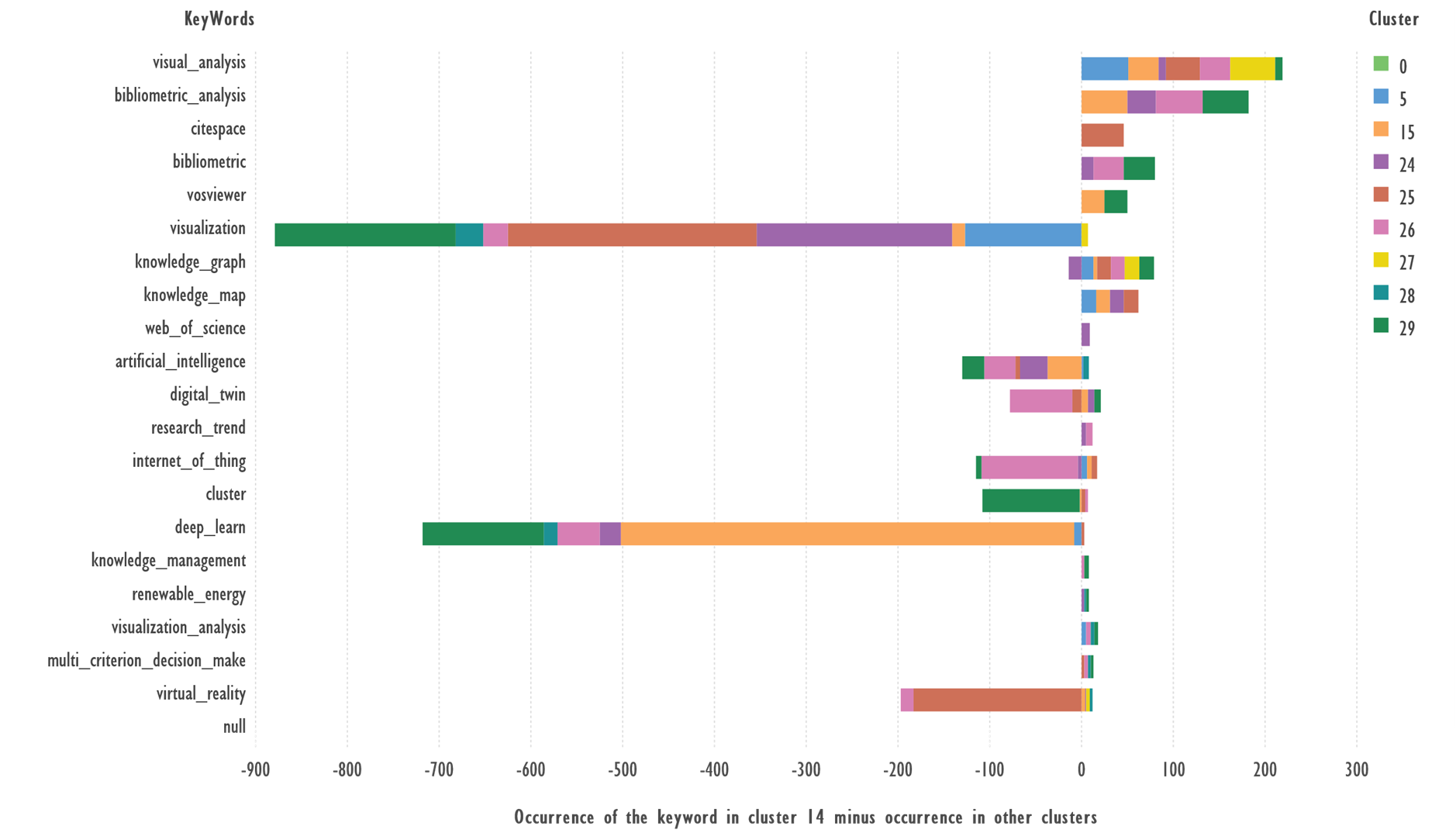
Fig. 3. Comparison of keywords from Cluster 14 and the rest of the clusters. Terms with 5 or more occurrences were used.

 

There are no keywords in this cluster that do not occur in other clusters.

Terms: ‘visual_analysis’, ‘bibliometric_analysis’, ‘citespace’, ‘bibliometric’, ‘vosviewer’, ‘knowledge_map’, ‘web_of_science’ which occur more frequently in cluster 14 than in other clusters, can serve as candidates to describe the cluster theme; ‘visualization’, ‘deep_learn’, ‘virtual_reality’ are more likely to occur in other clusters.

Figure 4 shows the difference between the occurrence of the most frequent keywords in Cluster 15 and the other clusters.

 

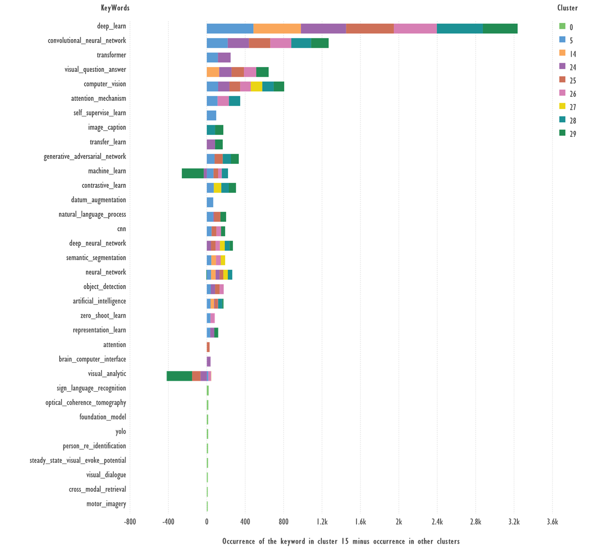
Fig. 4. Comparison of keywords from Cluster 15 and the rest of the clusters. Terms with 39 or more occurrences were used.

 

Terms: ‘sign_language_recognition → 19’, ‘optical_coherence_tomography → 16’, ‘foundation_model → 14’, ‘yolo → 14’, ‘person_re_identification → 13’, ‘steady_state_visual_evoke_potential → 13’, ‘visual_dialogue → 11’, ‘cross_modal_retrieval → 10’, ‘motor_imagery → 10’ occurs less than 39 times, but added to the figure to make it more fully understood.

Terms: ‘deep_learn’, ‘convolutional_neural_network’, ‘transformer’, ‘visual_question_answer’, ‘computer_vision’, ‘attention_mechanism’, ‘generative_adversarial_network’, ‘contrastive_learn’ which occur more frequently in cluster 15 than in other clusters, can serve as candidates to describe the cluster theme; ‘machine_learn’, ‘visual_analytic’ are more likely to occur in other clusters.

Figure 5 shows the difference between the occurrence of the most frequent keywords in Cluster 24 and the other clusters.

 

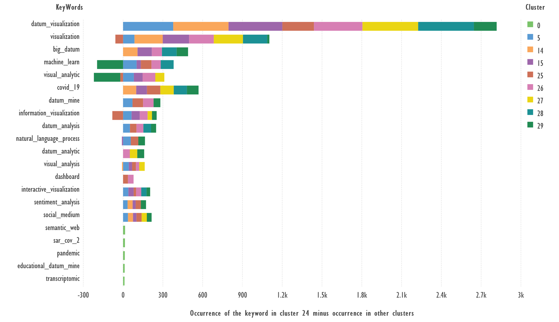
Fig. 5. Comparison of keywords from Cluster 24 and the rest of the clusters. Terms with 40 or more occurrences were used.

 

Terms: ‘semantic_web 15’, ‘sar_cov_2 14’, ‘pandemic 13’, ‘educational_datum_mine 12’, ‘transcriptomic 11’ occurs less than 40 times, but added to the figure to make it more fully understood.

Terms: ‘datum_visualization’, ‘big_datum’, ‘covid_19’, ‘datum_mine’, ‘datum_analysis’, ‘interactive_visualization’, ‘sentiment_analysis’, ‘sentiment_analysis’, ‘social_medium’ which occur more frequently in cluster 24 than in other clusters, can serve as candidates to describe the cluster theme; ‘machine_learn’, ‘visual_analytic’ are more likely to occur in other clusters. Topic ‘covid_19’ has been analyzed extensively in scientific publications.

Figure 6 shows the difference between the occurrence of the most frequent keywords in Cluster 25 and the other clusters.

 

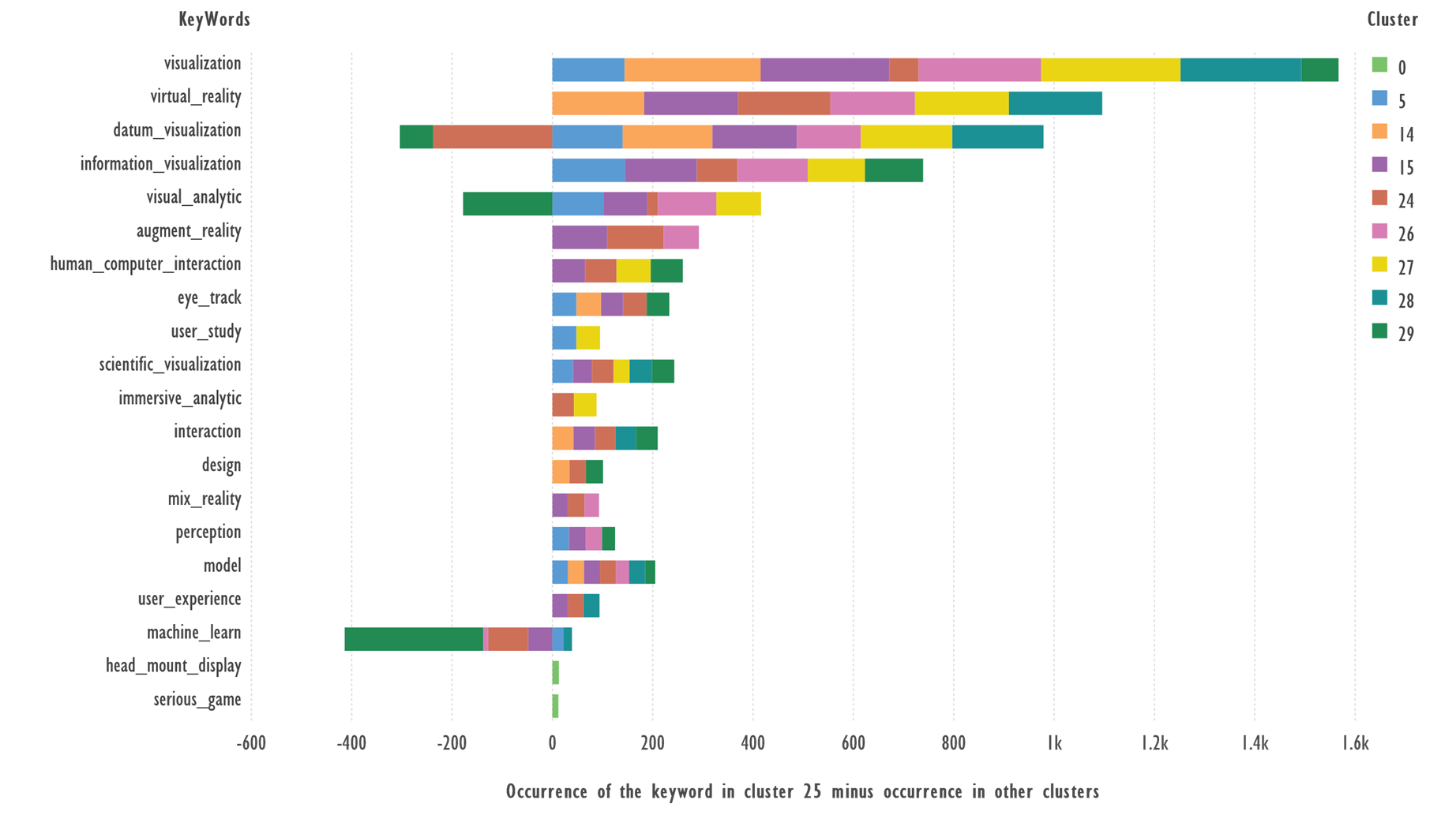
Fig. 6. Comparison of keywords from Cluster 25 and the rest of the clusters. Terms with 32 or more occurrences were used.

 

Terms: ‘head_mount_display 13’, ‘serious_game  12’, occurs less than 32 times, but added to the figure to make it more fully understood.

Terms: ‘visualization’, ‘virtual_reality’, ‘information_visualization’, ‘augment_reality’, ‘human_computer_interaction’, ‘eye_track’, ‘scientific_visualization’, ‘immersive_analytic’, ‘interaction’ which occur more frequently in cluster 25 than in other clusters, can serve as candidates to describe the cluster theme; ‘machine_learn’ occur in other clusters.

Figure 7 shows the difference between the occurrence of the most frequent keywords in Cluster 26 and the other clusters.

 

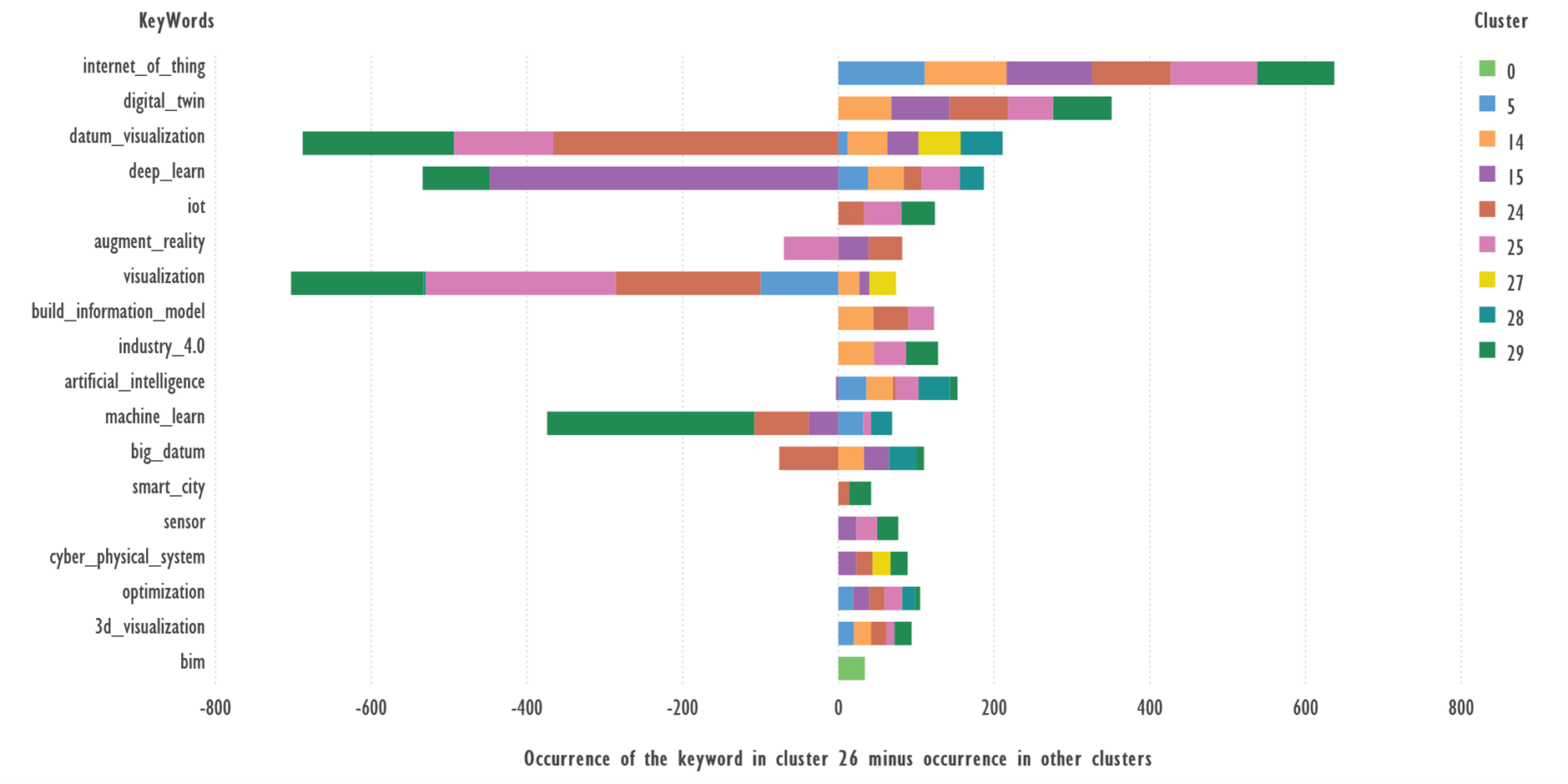
Fig. 7. Comparison of keywords from Cluster 26 and the rest of the clusters. Terms with 23 or more occurrences were used.

 

Terms: ‘internet_of_thing’, ‘digital_twin’, ‘iot’, ‘build_information_model’, ‘industry_4.0’, ‘artificial_intelligence’, ‘cyber_physical_system’, ‘optimization’, ‘3d_visualization’ which occur more frequently in cluster 26 than in other clusters, can serve as candidates to describe the cluster theme; ‘datum_visualization’, ‘deep_learn’, ‘visualization’, ‘machine_learn’ occur in other clusters.

Note: No abbreviation substitution was used in the preparation of the texts, so ‘internet_of_thing’ and ‘iot’ are marked as different terms. It is useful to compile a list of thematic abbreviations for use in future work.

Figure 8 shows the difference between the occurrence of the most frequent keywords in Cluster 27 and the other clusters.

 

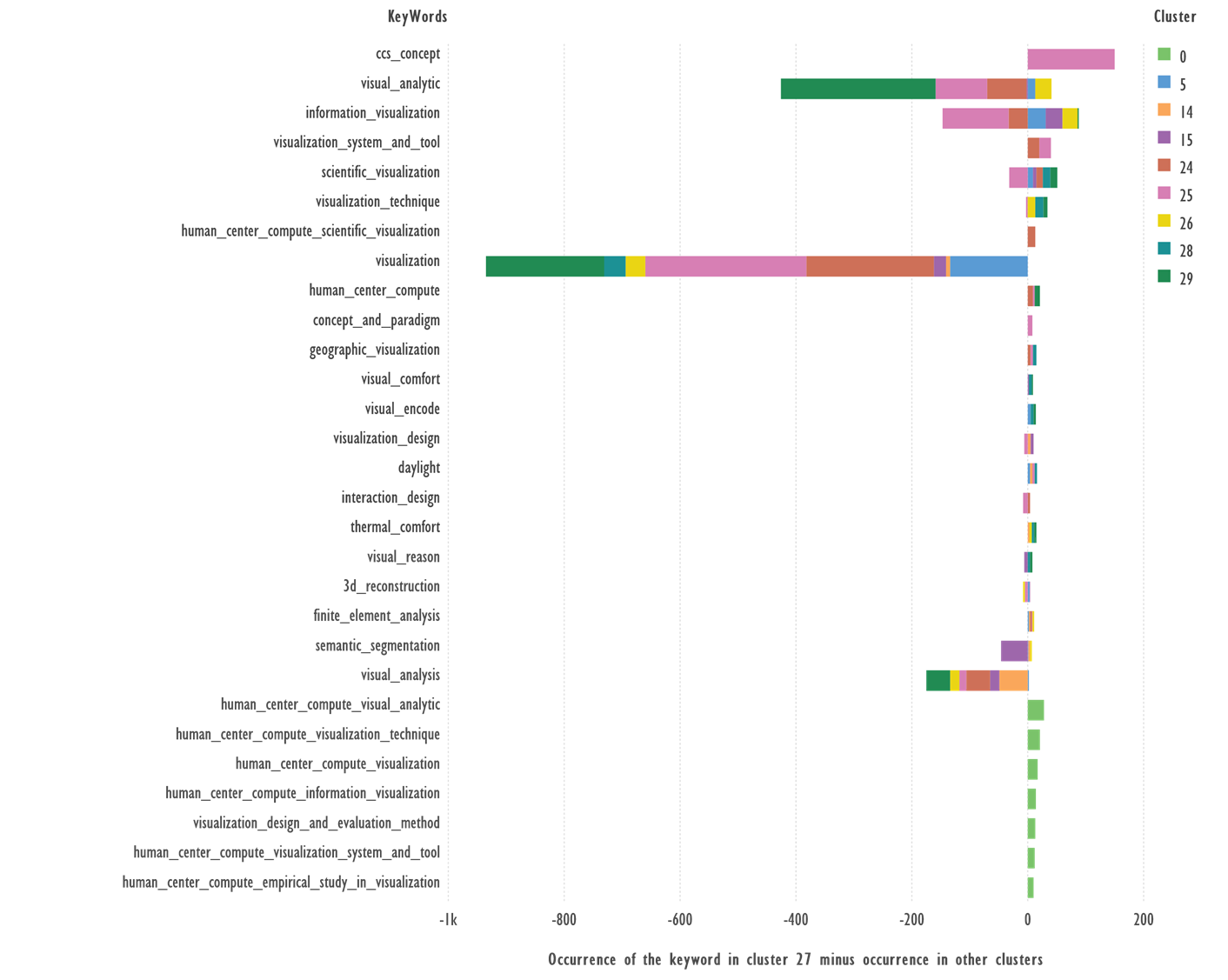
Fig. 8. Comparison of keywords from Cluster 27 and the rest of the clusters. Terms with 4 or more occurrences were used.

 

Terms: ‘human_center_compute_visual_analytic’, ‘human_center_compute_visualization_technique’, ‘human_center_compute_visualization’, ‘human_center_compute_information_visualization’, ‘visualization_design_and_evaluation_method’, ‘human_center_compute_visualization_system_and_tool’, ‘human_center_compute_empirical_study_in_visualization —occur only in cluster 27, reflecting the specificity of the cluster topic.

Terms: ‘ccs_concept’, ‘information_visualization’, ‘visualization_system_and_tool’, ‘visualization_technique’, ‘human_center_compute_scientific_visualization’ which occur more frequently in cluster 14 than in other clusters, can serve as candidates to describe the cluster theme; ‘visual_analytic’, ‘visualization’, ‘visual_analysis’ occur in other clusters.

Figure 9 shows the difference between the occurrence of the most frequent keywords in Cluster 28 and the other clusters.

 

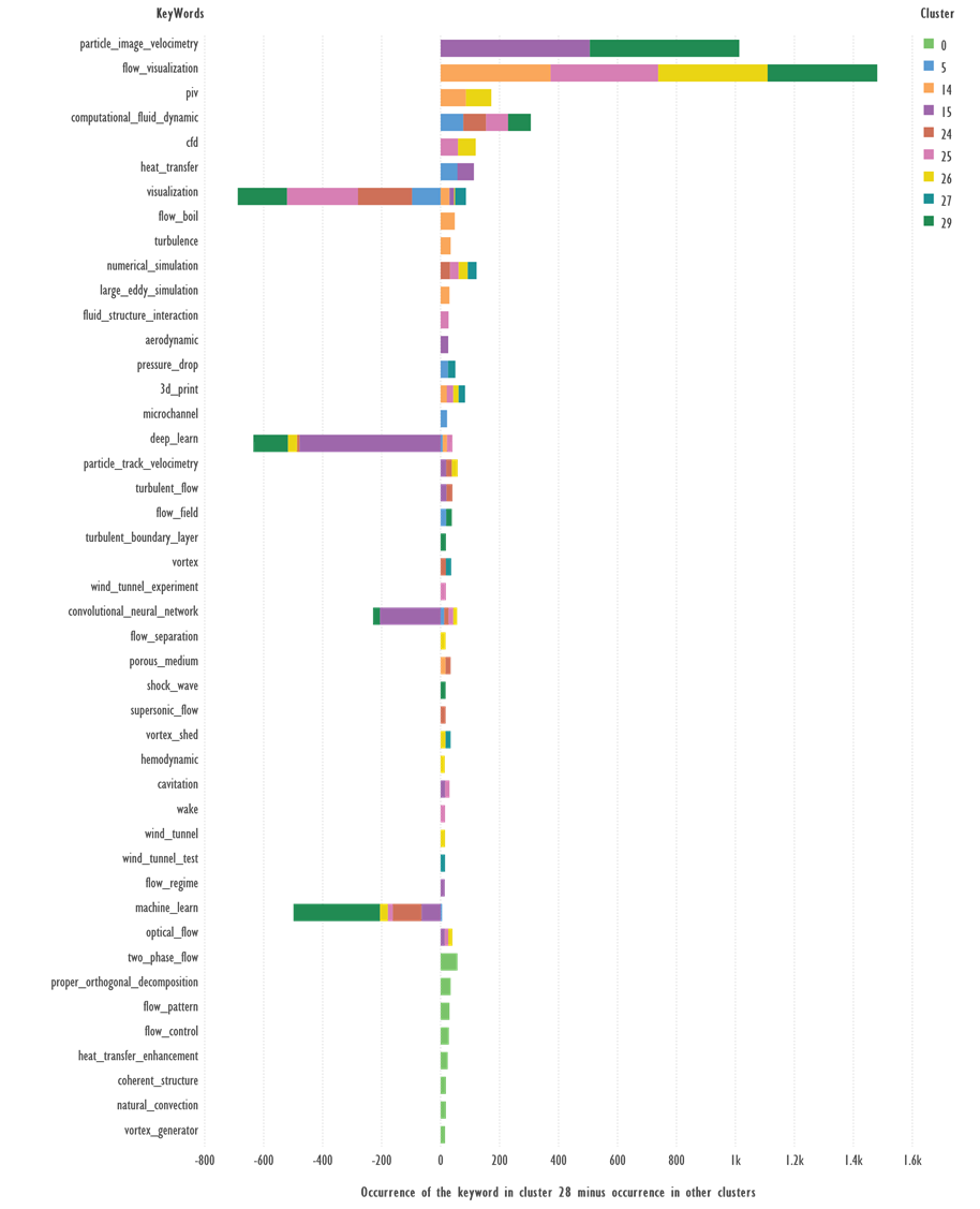
Fig. 9. Comparison of keywords from Cluster 28 and the rest of the clusters. Terms with 15 or more occurrences were used.

 

Terms: ‘two_phase_flow’, ‘proper_orthogonal_decomposition’, ‘flow_pattern’, ‘flow_control’, ‘heat_transfer_enhancement’, ‘coherent_structure’, ‘natural_convection’, ‘vortex_generator’ —occur only in cluster 28, reflecting the specificity of the cluster topic.

Terms: ‘particle_image_velocimetry’, ‘flow_visualization’, ‘piv’, ‘computational_fluid_dynamic’, ‘cfd’, ‘heat_transfer’, ‘flow_boil’, ‘turbulence’, ‘numerical_simulation’, ‘3d_print’ which occur more frequently in cluster 28 than in other clusters, can serve as candidates to describe the cluster theme; ‘visualization’, ‘deep_learn’, ‘convolutional_neural_network’ occur in other clusters.

Figure 10 shows the difference between the occurrence of the most frequent keywords in Cluster 29 and the other clusters.

 

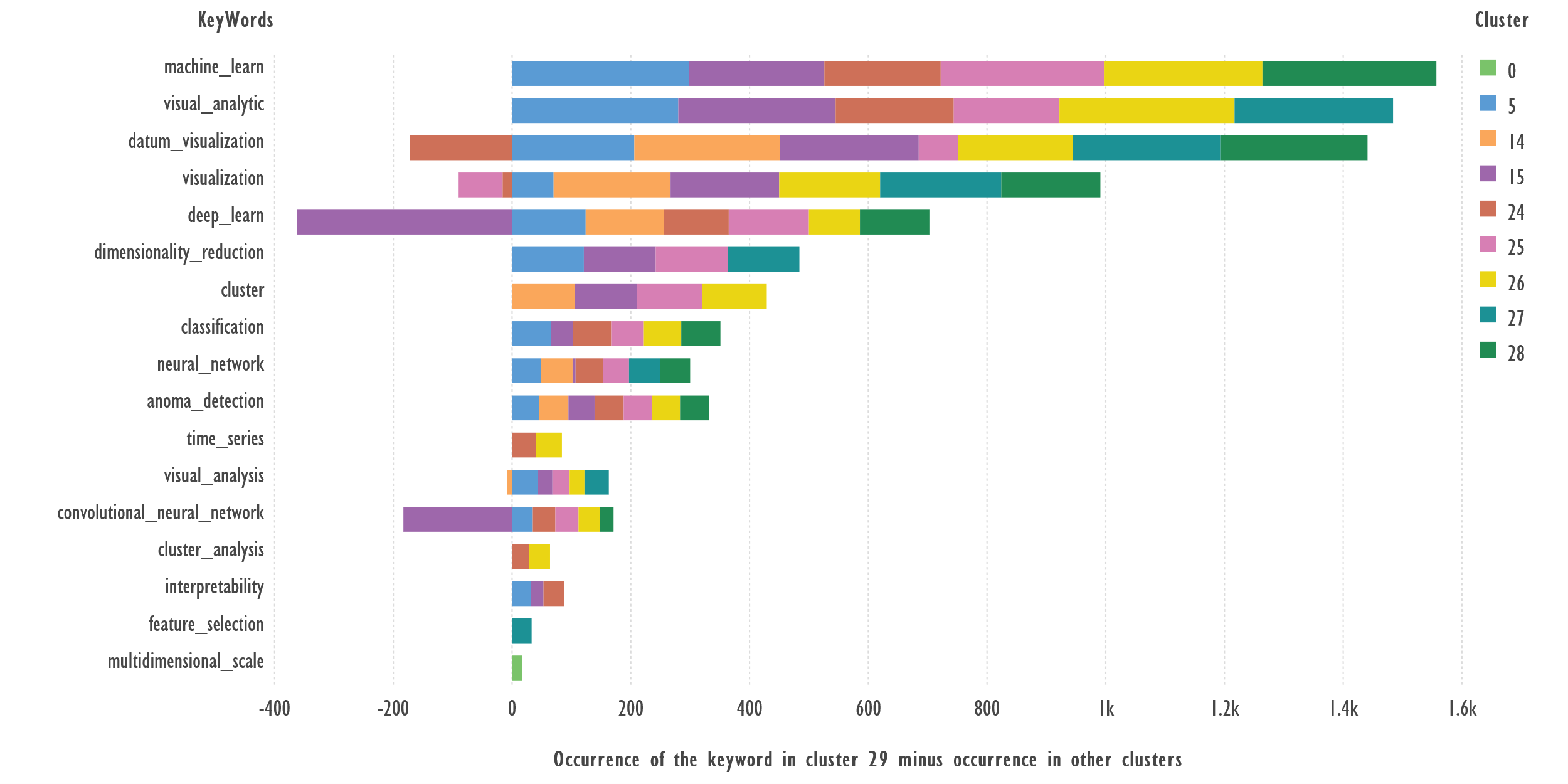
Fig. 10. Comparison of keywords from Cluster 29 and the rest of the clusters. Terms with 34 or more occurrences were used.

 

Term: ‘multidimensional_scale’ — occurs only in cluster 29, reflecting the specificity of the cluster topic.

Terms: ‘machine_learn’, ‘visual_analytic’, ‘dimensionality_reduction’, ‘cluster’, ‘classification’, ‘neural_network’, ‘anoma_detection’, ‘time_series’, ‘visual_analysis’, ‘cluster_analysis’, ‘interpretability’, ‘feature_selection’ which occur more frequently in cluster 29 than in other clusters, can serve as candidates to describe the cluster theme; ‘deep_learn’, ‘convolutional_neural_network’ — frequently appear in cluster 15.

3.2 Comparison of Author keywords in VOSviewer and GSDMM clusters

In bibliometric analysis, keyword clustering using VOSviewer software is more commonly used rather than document clustering using GSDMM.

Thus, the simplest query to the open abstract database ScienceDirect ‘document clustering gsdmm’ gives only 40 publications, the query ‘Gibbs Sampling’ ‘Dirichlet Multinomial Mixture’ — 60 results, and the query ‘keyword clustering VOSviewer’ returns 4,570 results.

Therefore, it is interesting to compare the Author keywords clusters obtained with the VOSviewer program and the Author keywords specific to the record/document clusters obtained with the GSDMM algorithm. The approaches are quite different, but even an approximate overlap of dominant themes can indicate the semantic meaningfulness of the results obtained by the different methods.

For this comparison, the same prepared Author keywords records used in clustering with the GSDMM algorithm were imported into the VOSviewer software and a co-occurrence network of terms was constructed. The results are shown in Figure 11.

Using the default parameters, 13 clusters were obtained. In order to obtain an equal number of clusters to compare the results of the two approaches, the parameter reflecting the minimum number of keywords in a cluster was increased to 45.

 

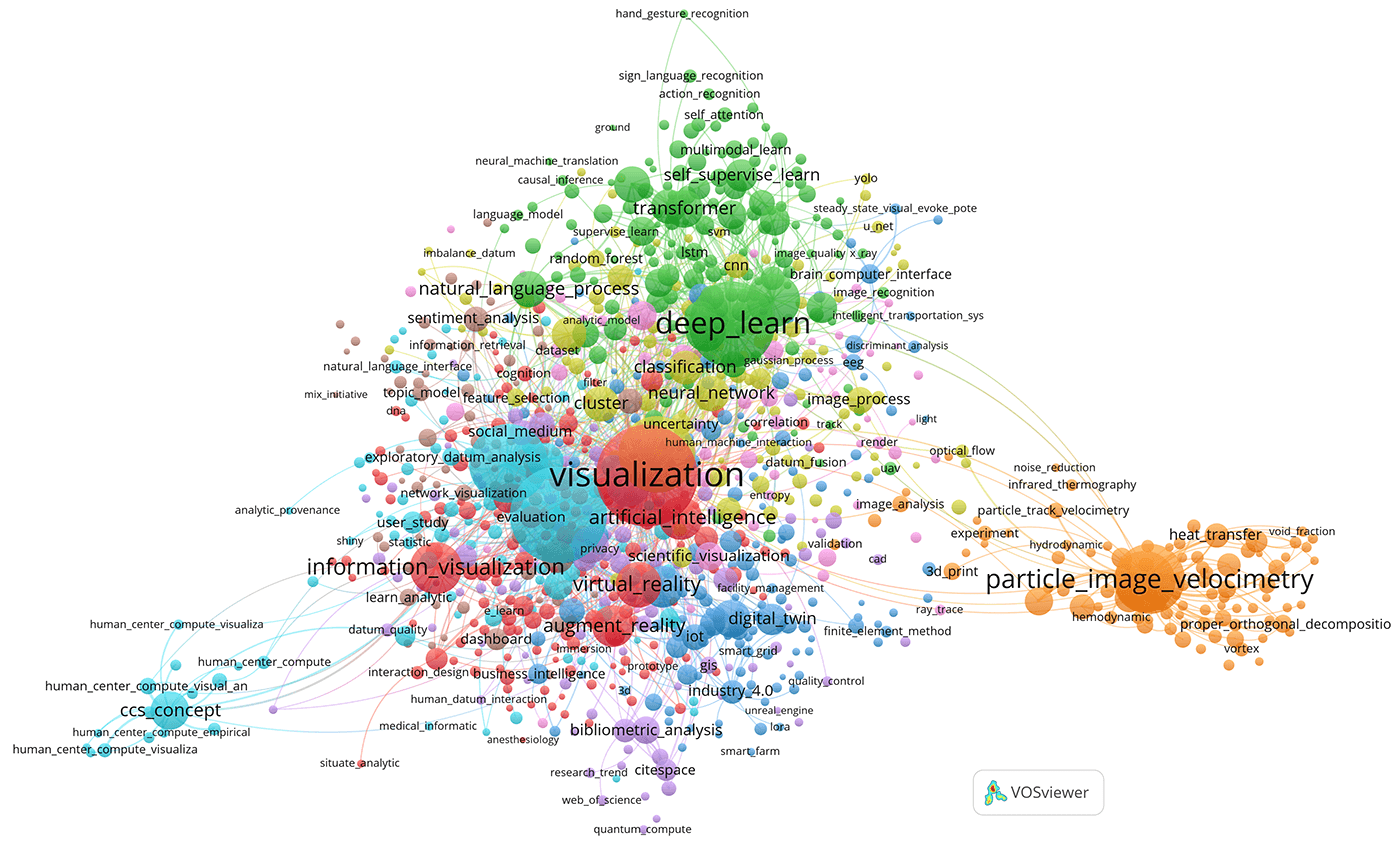
Fig. 11. Network of 9 clusters of co-occurrences of Author keywords. Obtained with the minimum number of terms in the cluster equal to 45.

 

The orange cluster, which can be tentatively called “particle_image_velocimetry”, stands out well in this figure; the terms of this cluster are also typical of the 28 cluster shown in Figure 9.

For a detailed examination of the results shown in Figure 11, the file ‘AuKWs16486-45-45-45.json’ included in the archive can be used at the service https://app.vosviewer.com/.

If we use the interactive features of the ‘app.vosviewer’ service, we can see that terms like ‘visualization’ or ‘deep_learn’ often co-occur with keywords from other clusters. Unlike document/record clustering, when clustering keywords, they belong to one cluster but may co-occur with keywords from other clusters.

The frequent occurrence of terms such as ‘visualization’ in different clusters of documents/records is quite understandable, as this term is included in the query for which data was collected in Scopus. Other common terms, such as ‘deep learning’, are not included in the query, but are often found in the broader context of papers about data.

The following is a brief comparison of keywords in clusters obtained using the GSDMM algorithm and the VOSviewer program. The aim is to find out the reproducibility of the identified topics obtained by significantly different methods.

The analysis was carried out as follows: for each cluster obtained by the two methods, a list of keywords and their occurrence was determined. From these lists, a sample of the 20 most frequent keywords was taken. The tables obtained were compared by INNER JOIN. The results of the comparison of the most similar tables are presented in Tables 1–10. Abbreviations in table titles: VOSviewer-AuKWs — author keywords from VOSviewer cluster; GSDMM-AuKWs — author keywords from GSDMM cluster. N — Number of Author Keywords in the cluster. VOSviewer Author Keywords can only belong to one cluster, while GSDMM Author Keywords can belong to several clusters, so they are not more than VOSviewer Author Keywords.

Table 1: INNER JOIN of top 20 terms from VOSviewer cluster 9 against top 20 terms from GSDMM cluster 5.

This table summarizes typical “task_analysis” steps. An example of the work could be [10].

Table 2: INNER JOIN of top 20 terms from VOSviewer cluster 5 against top 20 terms from GSDMM cluster 14.

This table shows: Visualization of bibliometric data is a relevant research topic. An example of the work could be [11].

Table 3: INNER JOIN of top 20 terms from VOSviewer cluster 2 against top 20 terms from GSDMM cluster 15.

The results of this table could be interpreted as follows: “convolutional_neural_network” is the most frequently encountered “deep_learn” method in studies on “computer_vision”. An example of the work could be [12]. And “transformer” and “natural_language_process” are the most frequent “visual_question_answer” methods in “visual_question_answer” studies.

Table 4: INNER JOIN of top 20 terms from VOSviewer cluster 6 against top 20 terms from GSDMM cluster 24.

Table 5: INNER JOIN of top 20 terms from VOSviewer cluster 8 against top 20 terms from GSDMM cluster 24.

In this case, two clusters obtained from VOSviewer were compared with data from a GSDMM cluster. In both tables, the topic is close to “data analysis”. An example of the work could be [13].

Table 6: INNER JOIN of top 20 terms from VOSviewer cluster 1 against top 20 terms from GSDMM cluster 25.

If we exclude terms of the general type “visualization” and “information_visualization”, the most characteristic terms of this table are “virtual_reality” and “augmented_reality”. An example of the work could be [14].

Table 7: INNER JOIN of top 20 terms from VOSviewer cluster 3 against top 20 terms from GSDMM cluster 26.

The term “iot” is an abbreviation for “internet_of_thing” they frequently occur in the records of the same cluster. This indicates the need to compile a dictionary of abbreviations, which, along with lemmatization, it is advisable to include in future works. An example of the work could be [15]. BIM (Building Information Model) is a rather specific term, so it has the same frequency of occurrence in the left and right columns.

Table 8: INNER JOIN of top 20 terms from VOSviewer cluster 6 against top 20 terms from GSDMM cluster 27.

The term visual_analytic occurs frequently in the bibliometric records used in this paper, it occurs 644 times in the VOSviewer cluster and only 37 times in the specific cluster of GSDMM, the rest of the occurrences of this term are in other GSDMM clusters. An example of the work could be [16].

Table 9: INNER JOIN of top 20 terms from VOSviewer cluster 7 against top 20 terms from GSDMM cluster 28.

In this case, the overlap of terms in the clusters is the highest of all 10 comparison tables. This is due to the fact that the cluster “particle_image_velocimetry” in the VOSviewer results is the most “freestanding”, i.e. its terms rarely co-occur with terms of other clusters. An example of an article reflecting the subject matter of this table is [17].

Table 10: INNER JOIN of top 20 terms from VOSviewer cluster 4 against top 20 terms from GSDMM cluster 29.

The terms machine_learn and neural_network are often found in combination with other terms, so their frequency is greater in the left column than in the right column. It is interesting to note that among the specific machine learning methods, random_forest is found in the table, which is often used in practical applications [18].

4. Conclusion

A technique for visualizing the results of Author keywords clustering by the GSDMM algorithm is proposed, which facilitates the evaluation of the topics of records/documents in the cluster. It is based on comparing the occurrence of keywords of a given cluster and other clusters.

It is shown that the topics of clusters obtained with GSDMM algorithm can be corresponded with the results of clustering of Author keywords performed with the use of VOSviewer program.

The obtained results can be interpreted as a certain stability of the themes of clusters obtained by essentially different methods.

For further development of this study, the author considers it appropriate to:

1. to compile a thematic dictionary of abbreviations that allows unambiguous interpretation of terms such as IoT and the Internet of Things;

2. extend the obtained method of visualizing clustering results to other short texts — titles and abstracts;

3. analyze the impact of dictionary compilation on the clustering results of the GSDMM algorithm.

Note. This work is mainly methodological. Its results will be used to identify promising research tasks to be carried out by the Institute and funded by the Ministry of Science and Higher Education of the Russian Federation.

Acknowledgments

The work was funded by the Ministry of Science and Higher Education of the Russian Federation (State Assignment No. FMME-2025-0012)

References

1. GitHub - MaartenGr/BERTopic: Leveraging BERT and c-TF-IDF to create easily interpretable topics. [Electronic resource] // GitHub. URL: https://github.com/MaartenGr/BERTopic (accessed: 23.01.2025).

2. McInnes L. lmcinnes/umap. Uniform Manifold Approximation and Projection [Electronic resource]. 2025. URL: https://github.com/lmcinnes/umap (accessed: 23.01.2025).

3. McInnes L., Healy J., Melville J. UMAP: Uniform Manifold Approximation and Projection for Dimension Reduction. arXiv, 2018. doi: 10.48550/ARXIV.1802.03426.

4. Wang M. et al. Vocabulary Matters: An Annotation Pipeline and Four Deep Learning Algorithms for Enzyme Named Entity Recognition // J. Proteome Res. 2024. Vol. 23, ¹ 6. P. 1915–1925. doi: 10.1021/acs.jproteome.3c00367.

5. Walker R. rwalk/gsdmm-rust [Electronic resource]. 2024. URL: https://github.com/rwalk/gsdmm-rust (accessed: 23.01.2025).

6. Kardos M. tweetopic: Blazing fast topic modelling for short texts. [Electronic resource]. 2022. URL: https://github.com/centre-for-humanities-computing/tweetopic (accessed: 23.01.2025).

7. Boudellioua I. Illias-b/Natural-Language-Processing [Electronic resource]. 2023. URL: https://github.com/Illias-b/Natural-Language-Processing (accessed: 23.01.2025).

8. Yin J., Wang J. A dirichlet multinomial mixture model-based approach for short text clustering // Proceedings of the 20th ACM SIGKDD international conference on Knowledge discovery and data mining. New York New York USA: ACM, 2014. P. 233–242. doi: 10.1145/2623330.2623715.

9. Hassan-Montero Y., De-Moya-Anegon F., Guerrero-Bote V.P. SCImago Graphica: a new tool for exploring and visually communicating data // EPI. 2022. P. e310502. doi: 10.3145/epi.2022.sep.02.

10. Elshehaly M. et al. QualDash: Adaptable Generation of Visualisation Dashboards for Healthcare Quality Improvement // IEEE Trans. Visual. Comput. Graphics. 2021. Vol. 27, ¹ 2. P. 689–699. doi: 10.1109/TVCG.2020.3030424.

11. Ding X., Yang Z. Knowledge mapping of platform research: a visual analysis using VOSviewer and CiteSpace // Electron Commer Res. 2022. Vol. 22, ¹ 3. P. 787–809. doi: 10.1007/s10660-020-09410-7.

12. Minaee S., Minaei M., Abdolrashidi A. Deep-Emotion: Facial Expression Recognition Using Attentional Convolutional Network // Sensors. 2021. Vol. 21, ¹ 9. P. 3046. doi: 10.3390/s21093046.

13. Camacho D. et al. The four dimensions of social network analysis: An overview of research methods, applications, and software tools // Information Fusion. 2020. Vol. 63. P. 88–120. doi: 10.1016/j.inffus.2020.05.009.

14. Yang Y. et al. Tilt Map: Interactive Transitions Between Choropleth Map, Prism Map and Bar Chart in Immersive Environments // IEEE Trans. Visual. Comput. Graphics. 2021. Vol. 27, ¹ 12. P. 4507–4519. doi: 10.1109/TVCG.2020.3004137.

15. Yu W. et al. A Global Manufacturing Big Data Ecosystem for Fault Detection in Predictive Maintenance // IEEE Trans. Ind. Inf. 2020. Vol. 16, ¹ 1. P. 183–192. doi: 10.1109/TII.2019.2915846.

16. Spinner T. et al. explAIner: A Visual Analytics Framework for Interactive and Explainable Machine Learning // IEEE Trans. Visual. Comput. Graphics. 2019. P. 1–1. doi: 10.1109/TVCG.2019.2934629.

17. Harte N.C. et al. Second order and transverse flow visualization through three-dimensional particle image velocimetry in millimetric ducts // Experimental Thermal and Fluid Science. 2024. Vol. 159. P. 111296. doi: 10.1016/j.expthermflusci.2024.111296.

18. Jiang F. et al. The controlling factors and prediction model of pore structure in global shale sediments based on random forest machine learning // Earth-Science Reviews. 2023. Vol. 241. P. 104442. doi: 10.1016/j.earscirev.2023.104442.